Antichains and Dilworth’s Theorem

There’s lots of different possible definitions of “width” for a directed acyclic graph. For an app I’m developing, I wanted a simple way to measure how far from linear a DAG is, with the constraint that it generalizes my intuition that the width of a directed tree is the number of leaves. The definition I settled on is the maximum antichain size, where an antichain for a DAG \(G\) is any set of nodes \(S\) such that for any distinct pair \(u, v \in S\), \(u \neq v\), there is no path from \(u\) to \(v\) in \(G\).

Okay, so how can this maximum-size antichain be found? First, we need Dilworth’s theorem, which states:

in any finite partially ordered set, the maximum size of an antichain of incomparable elements equals the minimum number of chains needed to cover all elements.

The theorem is talking about partially ordered sets (posets), not DAGs, but this works for our purpose because every DAG is secretly a poset: just take the transitive closure of the edge relation, and you get a strict partial order. Using this partial ordering language, another way to define an antichain is any set of nodes that are mutually incomparable under the DAG ordering.

We should also be specific about the second part of the theorem: the “chain cover”, or more precisely chain decomposition, is a partition of the node set into a collection of chains or totally ordered subsets.

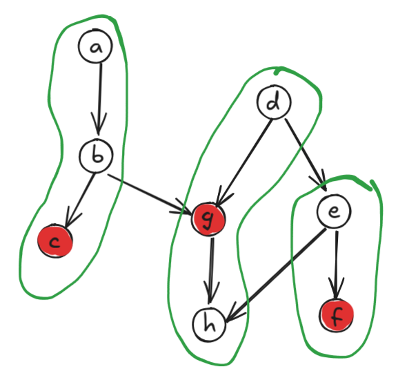
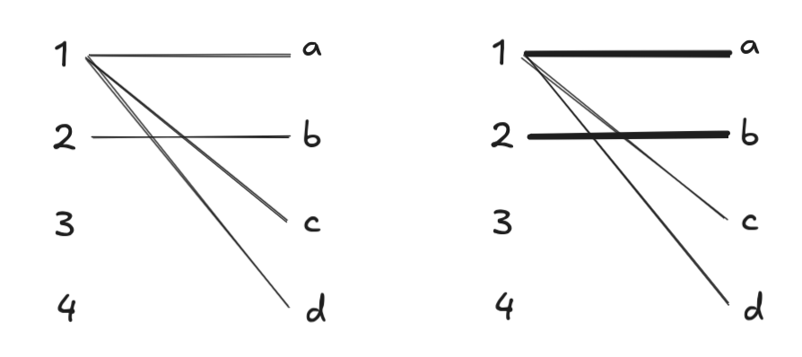
For example, I’ve drawn a DAG below as well as a minimum-size chain decomposition of size 3. This isn’t the only such chain decomposition, but there are no smaller decompositions. Note also that an antichain of size 3 is highlighted in red.

So thanks to Dilworth’s theorem, we just need to find the minimum size of a chain decomposition

DAG path covers and maximum cardinality matchings of bipartite graphs

Next, we need the idea of a vertex-disjoint path cover of a DAG: a set of paths in the DAG such that every node belongs to exactly one of the paths (i.e. the paths partition the node set).

We also need the notion of turning a DAG into a bipartite graph. This is done by making a new graph, \(B\), whose vertex set consists of the disjoint union of two copies of the nodes, \(L = G.V\) and \(R = G.V\), and whose edge set is formed by taking each \((u, v) \in G.E\) and drawing an edge from the copy of \(u\) in \(L\) to the copy of \(v\) in \(R\).

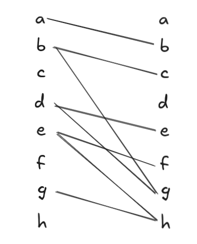
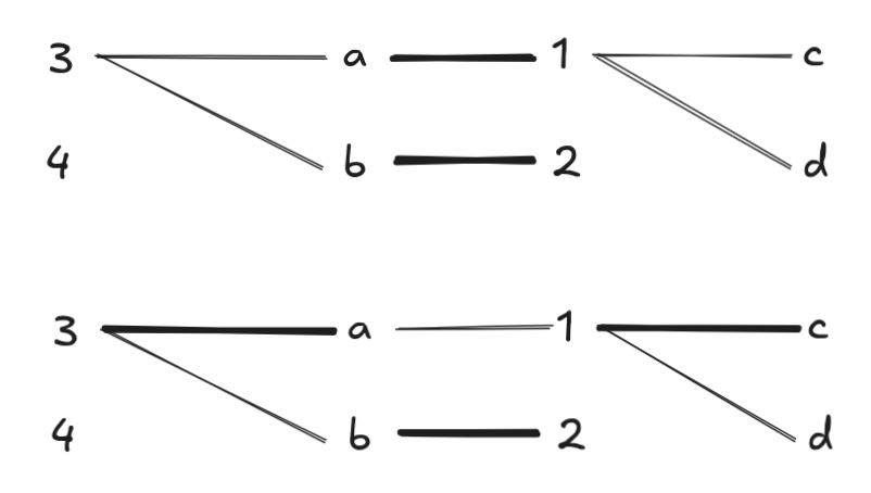
As an example, the above graph is transformed into this bipartite graph:

We bring the previous two ideas together with a third idea: a matching, or independent edge set: a set of edges such that no two edges share the same vertex. It turns out there is a fundamental relationship between vertex-disjoint path covers of a DAG and the maximum cardinality matching of the bipartite graph version of a DAG:

\[\boxed{\text{min vertex-disjoint path cover size of } G = |G.V| - \text{max matching size of } \text{Bip}(G)}\]

This is because every edge you add in the matching joins two paths that were previously separate, thereby reducing the number of paths in the path cover by 1. Initially there are |G.V| paths, each of consisting of a single node with no edges in it. Finding a matching of maximum cardinality among all matches is another way of saying you can construct a vertex-disjoint path cover of minimum cardinality.

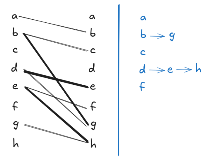
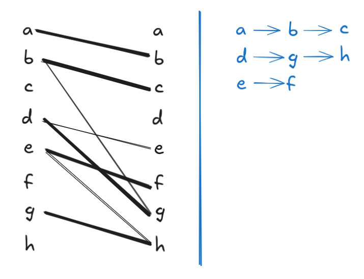
Note that the above matching is non-maximal: we can add \(a \to b\) to the matching to reduce the path cover size by 1. After this addition, however, we are stuck and can’t add any more edges, so the resulting matching is maximal. But \(|G.V| = 8\), and the resulting maximal matching has a size of 4, so the resulting vertex-disjoint path cover has a size of \(8 - 4 = 4\). But we already know from Figure 1 that there’s a path cover of size 3. Here the bipartite matching that produces it:

I included this example just to point out that we will need to be careful when trying to find a maximum matching: if we choose incorrectly, we can get stuck in a locally optimum matching that is not globally optimal.

Transitive closure DAGs

What is the max antichain size of the DAG below?

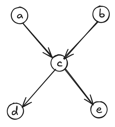
It’s clearly 2: either \(\{a, b\}\) or \(\{d, e\}\) work. But look at the corresponding chain decomposition:

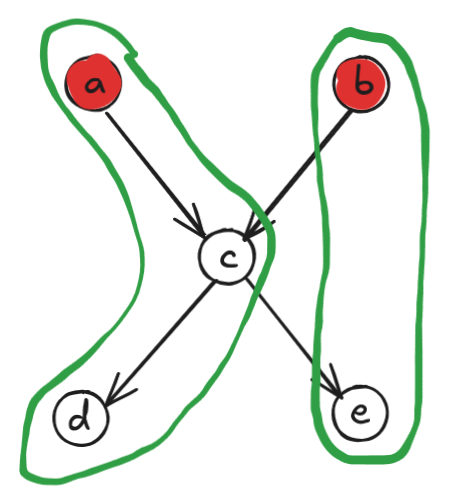
It may seem counterintuitive at first since we have chains \(a \to c \to d\) and \(b \to e\), but \(b\) and \(e\) are not directly connected! However, we have to remember that Dilworth’s theorem talks about partially ordered sets, not DAGs. Therefore, the graph we actually care about is the transitive closure graph:

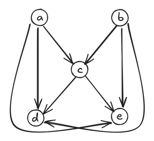
The transitive closure graph \(G^\ast\) is the graph with the same nodes as \(G\) and edges \((u, v)\) for all non-trivial paths from \(u\) to \(v\) in \(G\). Now the chains from our previous chain decomposition actually are paths in the transitive closure graph. More generally, since edges in \(G^\ast\) correspond to paths in \(G\), it’s easy to see that paths in \(G^\ast\) correspond to subsequences of paths in \(G\). In other words, paths in \(G^\ast\) are chains (totally-ordered subsets) under the DAG ordering.

Now apply the equation from the previous section:

\[\text{min vertex-disjoint path cover size of } G^\ast = |G.V| - \text{max matching size of } \text{Bip}(G^\ast)\]

Note that “vertex-disjoint path cover” of \(G^\ast\) is just a synonym for “chain decomposition”, for reasons just described. So what we have here is:

\[\boxed{\text{min chain decomposition size of } G^\ast = |G.V| - \text{max matching size of } \text{Bip}(G^\ast)}\]

To compute the width of a DAG, we simply need a way to efficiently compute the maximum cardinality matching of a bipartite graph.

Hopcroft-Karp algorithm

It turns out that the Hopcroft-Karp algorithm (see also here) does exactly this, and it runs in worst-case \(O(|E| \sqrt{|V|})\) time. My particular use case involves analyzing the BlueSky post graph, where each node can have at most two edges. This means \(|E| = O(2 |V|)\), so it runs in worst-case \(O(|V|^{1.5})\), which isn’t too terrible!

Important to the algorithm is the idea of an augmenting path. If you recall in Figure 3 there was a matching that was maximal but not maximum: we had to delete some of the edges in the matching in order to find a bigger matching. An augmenting path enables this kind of operation: it’s a path that starts at a free node (a node that is not part of any pair in the matching), ends at a free node, and for which the edges alternate (free edge, matching edge, free edge, …). Finding an augmenting path always increases the size of the matching: for every matching edge in the path, you remove it from the current matching, and for every free edge you add it to the current matching. There are, by construction, 1 more free edge than matching edge, so integrating an augmenting path always increases the matching size by one.

The algorithm doesn’t just find one augmenting path, it finds as many as possible: a maximal set of augmenting paths, which are vertex-disjoint from each other. The high-level pseudocode looks like this:

Hopcroft-Karp(B):

• \(M \leftarrow \emptyset\)
• while there is an augmenting path in \(B\):
  • \(P \leftarrow \text{maximal set of vertex-disjoint shortest augmenting paths}\)
  • \(M \leftarrow M \oplus P\)

The \(\oplus\) symbol above is the symmetric difference operator on sets.

Note that the requirement that we find the shortest augmenting paths is reminiscent of the Edmonds-Karp maximum flow algorithm. Because we want to find the shortest path, we first run a modified BFS starting from free nodes in \(L\). This sorts the graph into layers, which is used subsequently by multiple runs of DFS, again starting from free nodes in \(L\), to find the set of augmenting paths.

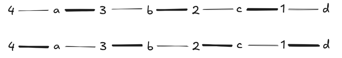
As a quick example, consider this bipartite graph (not from a DAG, just as an illustration):

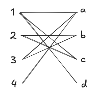
Running BFS, we find augmenting paths of length 1. Since \(\{a, b, c, d\}\) are all discovered before we explore from \(3\) or \(4\), BFS from these starting points terminates immediately. DFS produces the set of augmenting paths \(1 \to a\) and \(2 \to b\):

At this point, only \(3, 4 \in L\) are free nodes, so we run BFS from these start points. However, BFS from \(3\) visits all of \(4\)’s neighbors first, so it doesn’t find any augmenting paths involving \(4\). Two possible augmenting paths: \(3 \to a \to 1 \to c\) and \(3 \to a \to 1 \to d\) are found, and DFS picks the first one:

Now \(4\) is the only free node in \(L\), and BFS produces only one augmenting path, which DFS chooses. Note that we have to undo all previously selected pairs in the match at this point, which is why the augmenting path is so long:

Rough Python code is shown below:

from collections import deque

def hopcroft_karp(L, R, G):
    matching = {}
    dist = {}
    inf = float('inf')

    def bfs():
        q = deque()

        for n in L:
            if n not in matching:
                q.append(n)
                dist[n] = 0
            else:
                dist[n] = inf

        aug_path_found = False
        aug_path_length = inf
        while q:
            v = q.popleft()
            if dist[v] >= aug_path_length:
                break
            for n in G.get(v, []):
                # if n is free, we found an augmenting path
                n_partner = matching.get(n, None)
                if n_partner is None:
                    aug_path_length = dist[v] + 1
                    aug_path_found = True
                elif dist.get(n_partner, inf) == inf:
                    q.append(n_partner)
                    dist[n_partner] = dist[v] + 1
        return aug_path_found

    def dfs(u):
        for n in G.get(u, []):
            n_partner = matching.get(n, None)
            on_aug_path = n_partner is None or (dist.get(n_partner, inf) == dist[u] + 1
                and dfs(n_partner))
            if on_aug_path:
                matching[u] = n
                matching[n] = u
                return True
        return False

    matching_size = 0
    while bfs():
        for v in L:
            if v not in matching:
                if dfs(v):
                    matching_size += 1
    print(f"{matching_size=}")
    return matching

tl;dr

The final procedure is:

• Given a DAG \(G\), take its transitive closure \(G^\ast\)
• Convert \(G^\ast\) to a bipartite graph \(B\)
• Run Hopcroft-Karp on \(B\) to compute the size of the maximum matching, \(m\)
• Compute \(\text{width}(G) = |G.V| - m\)